DIJKSTRA

这个算法最开始设计出来并不是用来解决游戏中的寻路问题，而是来解决数学图形原理叫做最短路径。

这个方法一般在游戏寻路开发中使用的比较少，因为他是需要找到从开始点到结束点的所有路径，然后筛选出最短路径，这样做非常的浪费。

但是这是一个简单版本的A*算法，可以让我们更加容易的去理解A*。

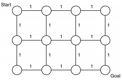
The Problem

我们需要找到一个最短路径，从开始点到目标点。

The Algorithm

粗略的概括这个算法就是，从起始节点根据它的连接线开始扩张。当它扩张的后面的节点时，我们需要记录下来，它是怎么来到这个节点的，我们可以反向画一个箭头，从当前节点指向上一个节点。这样我们就可以得到一个从前节点到当起始点的路径。最终我们到达目标节点，此时的路径就是我们所求得最短路径。

Processing the Current Node

这个算法使用迭代器来驱动，每一个迭代器记录着一个节点信息和连接这个节点的所有连接信息。

节点信息中有：上一个节点到节点的连接信息，从起始点到节点所有的花销

连接信息中有：头节点，尾节点和花销。

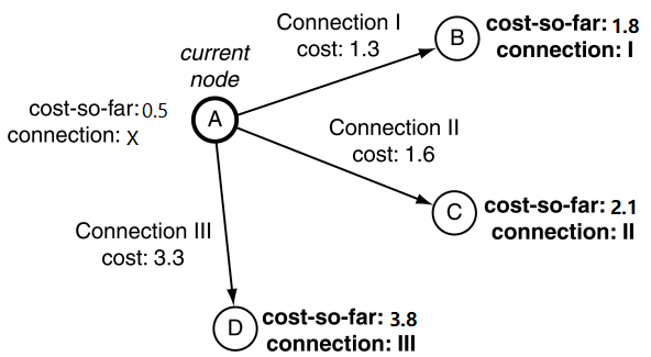
在上图中，对于第一个迭代器，开始节点就是当前节点。也就是说对于所有A点的连接的尾节点的总共花销就是对应每个连接的花销。

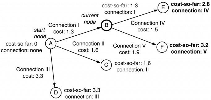
在上图中，当前节点是B时，B的每个连接的尾节点的总共花销等于当前连接的花销加上B节点的总共花销。

即：E的总共花销 = B到E的花销 + B节点的总共花销

The Node Lists

我们使用两个列表来记录已经被发现的节点：

• open ：已经发现了的节点，并未遍历到的节点（未处理的节点），我们在处理当前节点时，当前节点所有连接的尾节点都应该属于open列表里。
• closed ：已经遍历过的节点（处理过的节点）。

在一张图中，所有的节点只有三种状态：

• 被发现的节点，还未遍历
• 已经遍历过的节点
• 未被发现的节点

Calculating Cost-So-Far for Open and Closed Nodes

当我们计算尾节点的总共花销时，尾节点如果已经是被发现的节点，那么这个尾节点他是具有总共花销值的。我们就需要比较以当前节点做连接的总共花销小还是之前的总共花销小，如果之前的花销小，那么我们就跳过当前尾节点，反之我们就需要更新尾节点的数据。

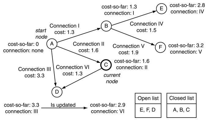
上图中，在最开始，我们就设置A->D的花销为3.3。当我遍历到C点时，计算C的尾节点D的总共花销等于连接VI的花销加上C的总共花销，也就是1.3+1.6=2.9。这个数值显然小于之前的3.3，所以我们需要更新D节点的迭代数据。

Terminating the Algorithm

当open列表里没有值时，这个算法就结束了，这时已经计算过从起始点到图中所有节点的路径，且所有节点都在closed列表里。

对于寻路，我们只关心到达目标节点，所以我们可以更早的结束遍历。

当前节点是目标节点时，我们就可以停止迭代。

但是很多时候，我们会在发现目标节点时，就停止迭代，即使我们获得的路径不是最短。因为在实际应用中最短的距离与发现目标节点时的那个路径差距并不大，所花去的时间差不多。

Retrieving the Path

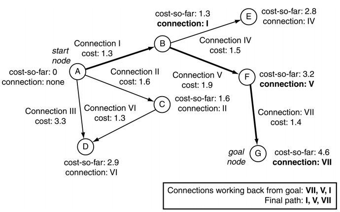
如上图，我们找到目标点G后，我们回溯G点的连接，再让他倒序即可获得路径。

Pseudo-Code

# This structure is used to keep track of the information we need
# for each node.
class NodeRecord:
    node: Node
    connection: Connection
    costSoFar: float
    
function pathfindDijkstra(graph: Graph, start: Node, end: Node) -> Connection[]:
    # Initialize the record for the start node.
    startRecord = new NodeRecord()
    startRecord.node = start
    startRecord.connection = null
    startRecord.costSoFar = 0

    # Initialize the open and closed lists.
    open = new PathfindingList()
    open += startRecord
    closed = new PathfindingList()

    # Iterate through processing each node.
    while length(open) > 0:
        # Find the smallest element in the open list.
        current: NodeRecord = open.smallestElement()

        # If it is the goal node, then terminate.
        if current.node == goal:
            break

        # Otherwise get its outgoing connections.
        connections = graph.getConnections(current)

        # Loop through each connection in turn.
        for connection in connections:
            # Get the cost estimate for the end node.
            endNode = connection.getToNode()
            endNodeCost = current.costSoFar + connection.getCost()

            # Skip if the node is closed.
            if closed.contains(endNode):
                continue

            # .. or if it is open and we’ve found a worse route.
            else if open.contains(endNode):
                # Here we find the record in the open list
                # corresponding to the endNode.
                endNodeRecord = open.find(endNode)
            if endNodeRecord.cost <= endNodeCost:
                continue

            # Otherwise we know we’ve got an unvisited node, so make a
            # record for it.
            else:
                endNodeRecord = new NodeRecord()
                endNodeRecord.node = endNode

            # We’re here if we need to update the node. Update the
            # cost and connection.
            endNodeRecord.cost = endNodeCost
            endNodeRecord.connection = connection

            # And add it to the open list.
            if not open.contains(endNode):
                open += endNodeRecord

    # We’ve finished looking at the connections for the current
    # node, so add it to the closed list and remove it from the
    # open list.
    open -= current
    closed += current

    # We’re here if we’ve either found the goal, or if we’ve no more
    # nodes to search, find which.
    if current.node != goal:
        # We’ve run out of nodes without finding the goal, so there’s
        # no solution.
        return null

    else:
        # Compile the list of connections in the path.
        path = []

     # Work back along the path, accumulating connections.
    while current.node != start:
        path += current.connection
        current = current.connection.getFromNode()

    # Reverse the path, and return it.
    return reverse(path)

Data Structures and Interfaces

Simple List

用来存储最后找到的路径，可以使用链表(std::list)或者变长数组(std::vector)

Pathfinding List

用来存储open和close列表，这两个列表对该算法非常重要，这直接关系到算法效率的好坏。这个列表主要有4个操作：

1. 添加节点到列表
2. 从列表中移除移除节点
3. 找到最小的花销的节点
4. 找到列表中中特殊的节点

我们需要合理的找到一个数据结构来使用，我们会在A*的章节来详细讲解一下这些数据结构。

Graph

我们在前面的实现也可以看到图的一些接口。

其中getConnections是最重要的一个方法，同时也是对性能影响至关重要。最常见的实现是：有一个存储的查询表并且使用节点的索引来查询。一个索引对应的是一个连接的数组。

连接的数据结构大概是这样的：

class Connection:
    cost: float
    fromNode: Node
    toNode: Node

    function getCost() -> float:
        return cost

    function getFromNode() -> Node:
        return fromNode

    function getToNode() -> Node:
        return toNode

Peformance of Dijkstra

该算法在内存和速度最大的依赖是操作寻路列表的数据结构，也就是open和close列表。

图中所有节点的个数为n，平均每个节点的连接数为m。那么这个算法的时间复杂度为O(nm)。

在算法结束时，有n个节点在close列表中，不会有超高nm个节点在open列表中。实际上在open列表里肯定会少于n个。所以最差情况下空间复杂O(nm)。

加上操作数据结构的时间，最差肯定会超过O(nm)。当然空间复杂度也会超过。

Weaknesses

该算法最大的劣势是不假选择的搜索整个图来找到最短的路径。

我们可以通过典型运行在不同阶段显示当前打开和关闭列表上的节点来可视化算法的工作方式。

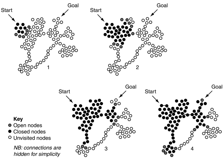
在每种情况下，搜索的边界都由开放列表上的节点组成。因为靠近开始点已经被处理过了。

可以看到最后一个图，找到了最短路径，也就是那根线。同时也发现了有很多离那根线很远的点，我们也处理了。这也增加了很多计算时间。

我们需要有选择性的去处理节点。